Summary
Get the app
In order to install the application, it first requires to download the application Urba Khroma from this website. Click on the Download section to enter the download page. Then download one of the two versions of the application according to your operating system: Windows or MacOS (the Linux version is not already released).
Install on Windows
First you need to download the application (see Get the App section above). During the downloading, you may encounter some alert messages. Please ignore them and proceed the installation as shown below.
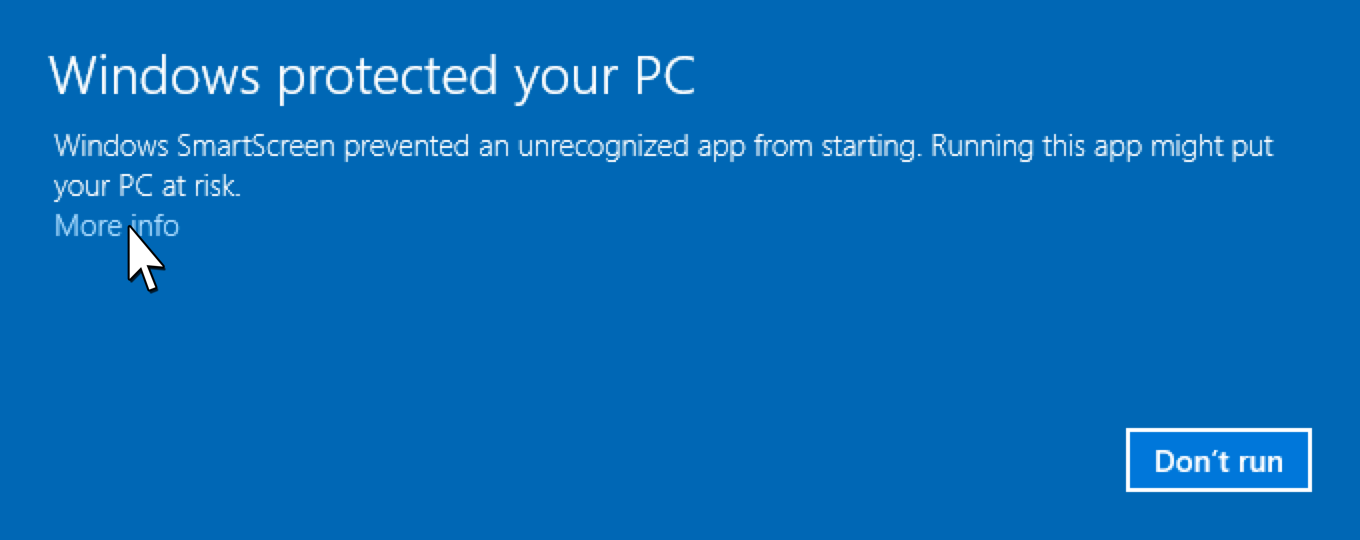
When the application is downloaded, the internet browser may block it by security. Please run it anyway.

On Windows 10:
Windows 10 has an additional security. Please ignore the warning by clicking on More info.
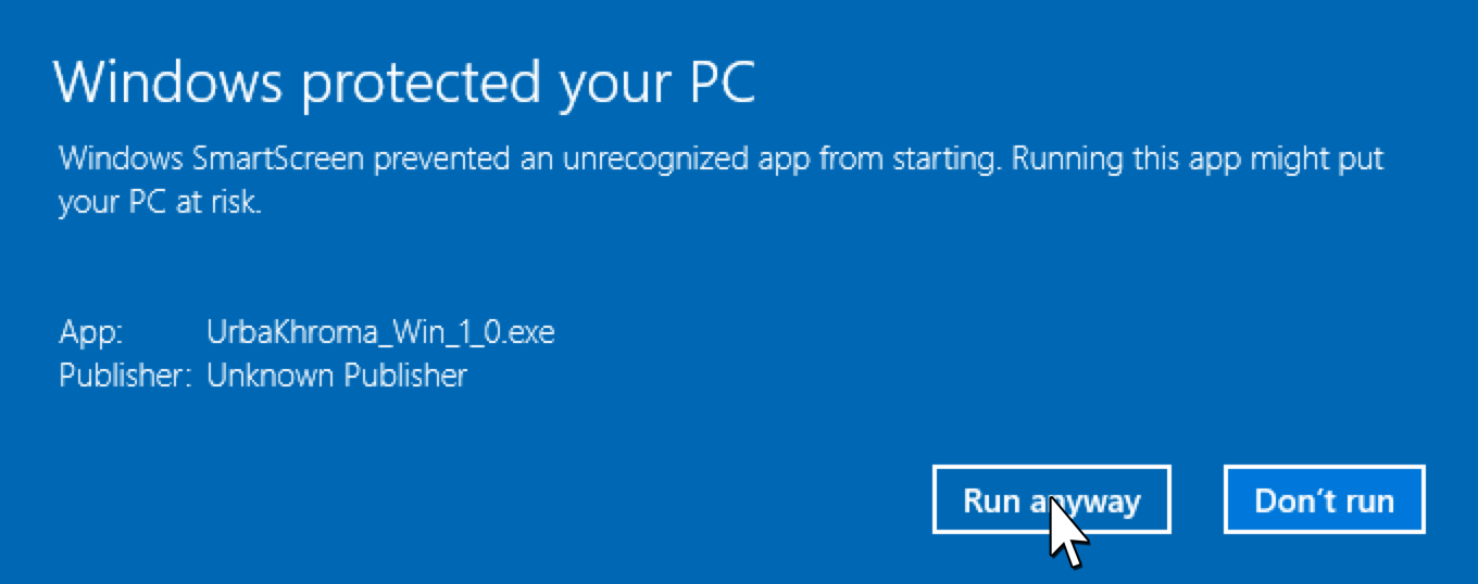
A new button Run anyway appears. Click on it.
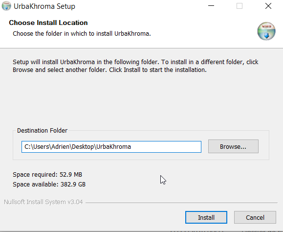
The installer opens. Select the installation folder for UrbaKhroma.
The installation in complete. You can run UrbaKhroma and create a desktop shortcut.
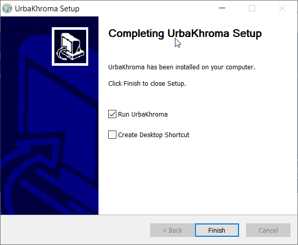
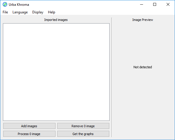
Finally, the application starts.
Install on MacOSX
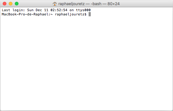
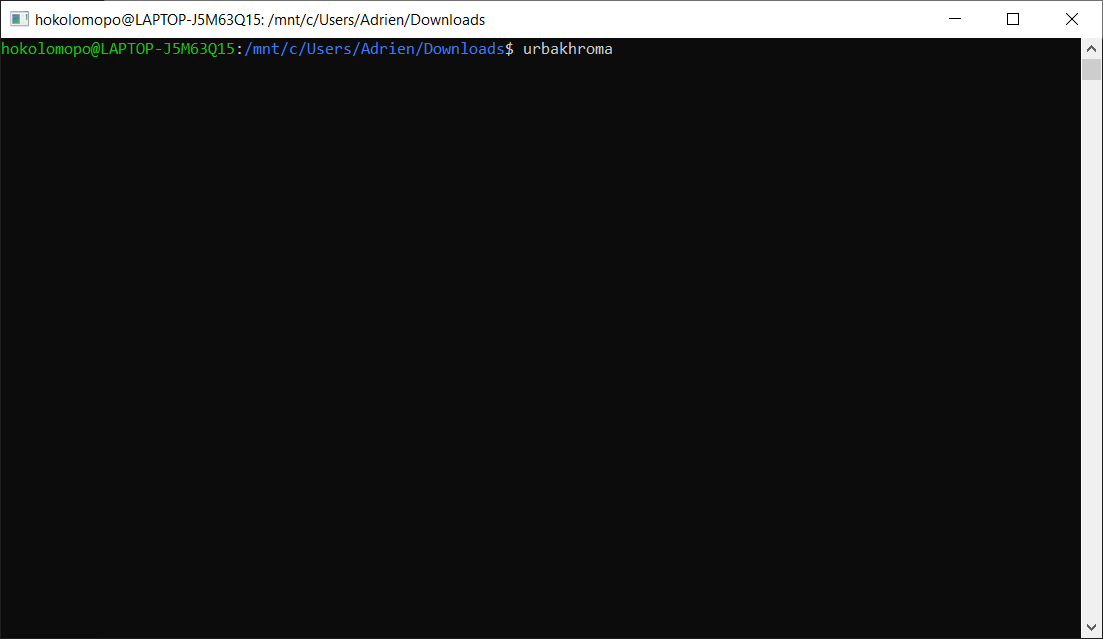
In order to run the application on MacOS, an additional component needs to be installed. The additional library that is needed is openCV. To ease the installation of that library, we will install this library through the terminal (in MacOS by default). To open the terminal on your Mac, go to Application/Utilities and double-click on Terminal.app (or do a quick-seach by pressing cmd+space and typing "terminal" on the search bar, then press enter). A white window appears.
In that terminal (the white window), we will write text command that will automatically install openCV in your Mac. The terminal may sometime asks your password to authenticate the installation. Please enter the password you use to start your computer (when typing password, there is no *** appearing, it is normal).
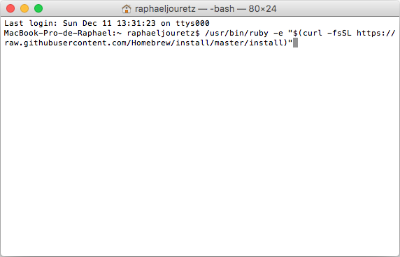
The first command to write inside the terminal is:
/usr/bin/ruby -e "$(curl -fsSL https://raw.githubusercontent.com/Homebrew/install/master/install)"
Copy-Paste this command in the terminal (right-click copy then right-click paste or cmd+c then cmd+v). You will get:
Type Enter. Some text will appears in the terminal. When the terminal asks
Press RETURN to continue or any other key to abort
press Enter again.
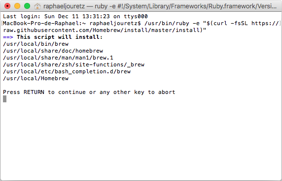
Some text will again appear. After five minutes you get (errors during the process could occur, please ignore them):
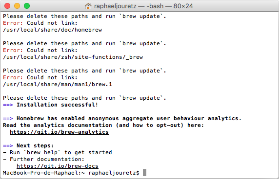
The first command was correctly executed using the terminal. We will now do the same for the second and the third command. First, copy this second command into the terminal as we did before:
brew tap homebrew/science
Then press Enter. Some text will again appear. Quickly, you will get:
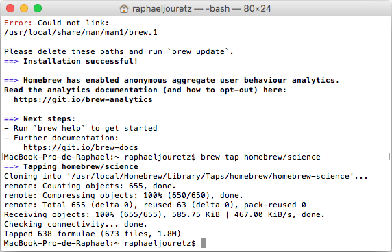
Finally, copy the last command to the terminal:
brew install opencv
And type Enter.. This last step will take a while. Please be patient...
When it is done, the last text the terminal has written is your name followed by $. In my case, it is:
MacBook-Pro-de-Raphael:~ raphaeljouretz$.
You can now close the terminal.
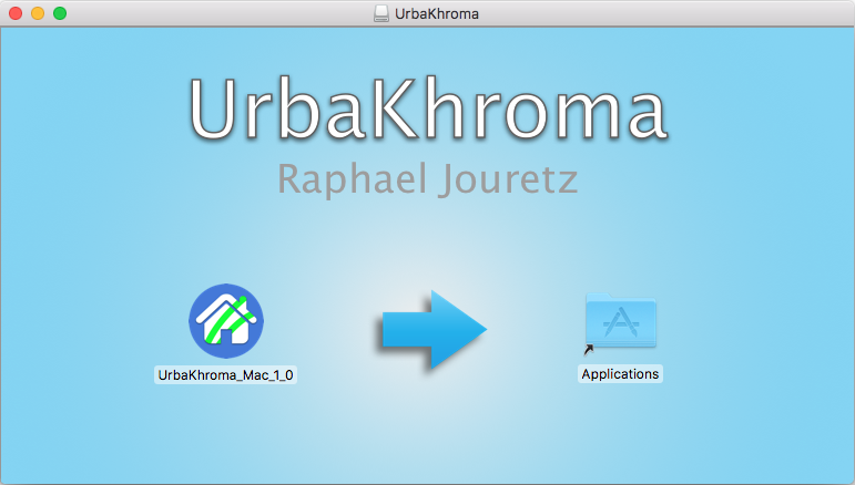
Now download the application from the Download section. Once downloaded, double-click on the downloaded file (UrbaKhroma_Mac_x_x.dmg). A window opens.
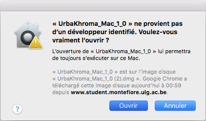
Right-click on UrbaKhroma_Mac_x_x and select Open.
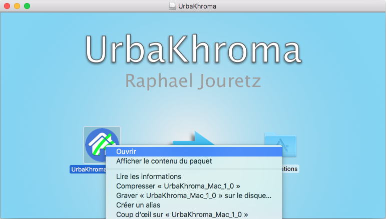
Finally, select Open again.
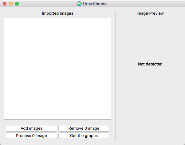
Here you are, you succesfully opened UrbaKhroma on your Mac.
The steps above are required only once, the first time you run the application. The next time you want to launch the application, just double-click on the UrbaKhroma_Mac_x_x inside the .dmg folder and the application automatically runs. You can also drag and drop the UrbaKhroma_Mac_x_x.app application inside your Application folder.
Install on Linux
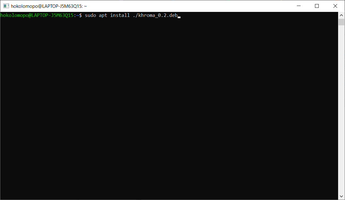
After downloading UrbaKhroma, open a terminal and go to the download folder.
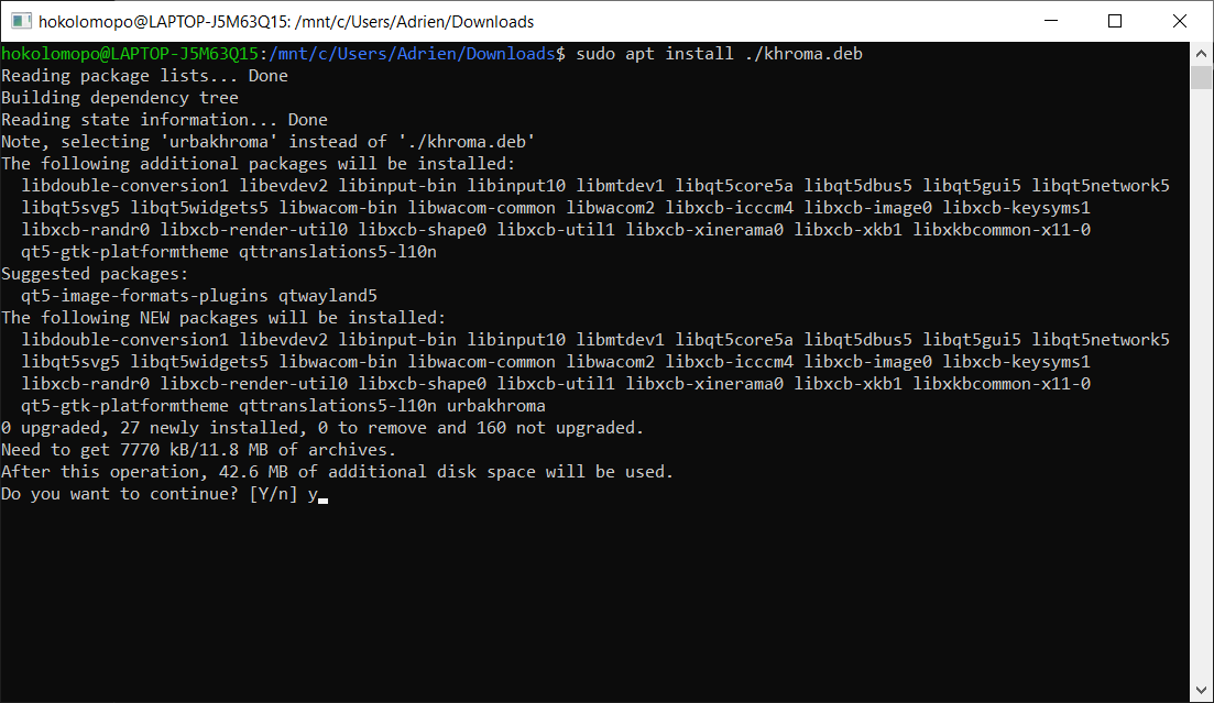
In the terminal, run this command to install the application (Replace apt by apt-get if you are using an older distribution of Ubuntu)
When prompted, type "y" and press enter. (If the installation fails, you may want to try to run the command "sudo apt update" and try again)
Run Urba Khroma with the "urbakroma" command.
Import Images
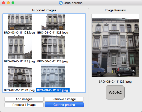
Since the application is used to get some statistic information about image colors, we need to import facade images inside the application. To do so, you can drag and drop images inside the Imported Images window or by clicking the Add Images button. Then browse the images you want to import into the project.
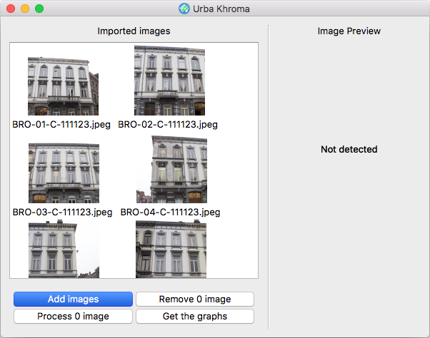
To remove images from the project, select the unwanted images from the Imported Images window and click on the Remove x Images button. Then click Yes on the message asking if you are sure to delete these images.
Extract Colors
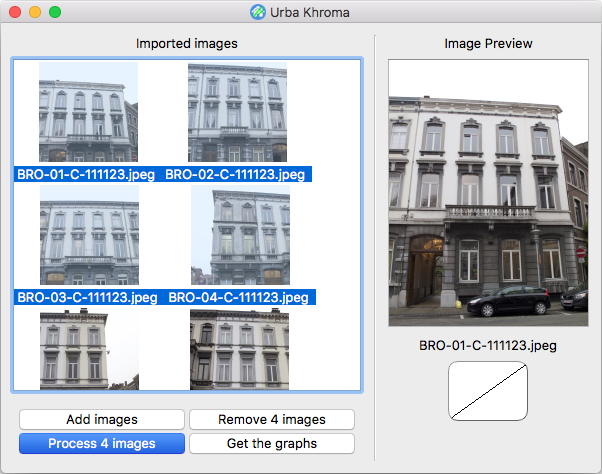
Now that you have imported images into the project, you need to analysed them, in order to extract colors from them. Inside the Imported Images window, select the image you want to extract and click on the Process x Images buttons.
1. Fill the gray chart.
The first step is the extraction of the gray chart that the photograph added on the picture. Since photos may be taken outside and the lighting conditions may influence the colors of the buildings, we put a standard reference on the picture to make a white balance.
To zoom on the image, use the zoom sliding bar. Once the image is focused on the gray chart, click on it with the mouse and fill it with green color.
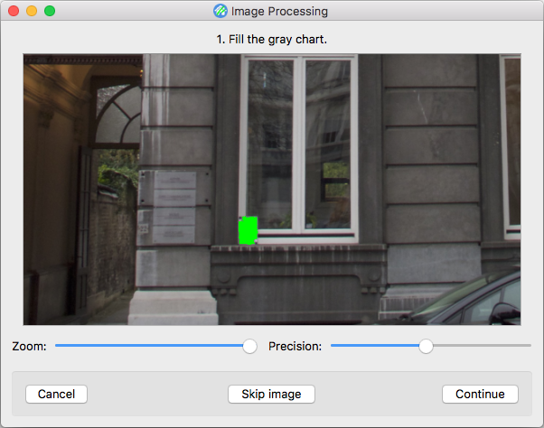
If the green color does not fill well the gray chart, you can modifiy the precision of the fill by sliding the cursor of the precision sliding bar.
If the image does not contain a gray chart, you can use the default gray chart by directly clicking on the continue button.
2. Select the 4 building corners.
The second step is the remove the background that can affect the facade color detection. To do so, click on the 4 corners of the buildings. At the fourth click, the background will be cut and only the picture inside the rectangle will remain.
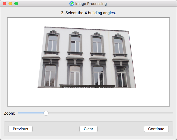
If the cut does not suit the building borders enough, click on the image to start again the selection or click on the Clear button.
3. Fill the zone to extract.
The last step is the extraction of the building facade color. The algorithm inside the program is semi-intelligent. It will analyze the image and recognize all the surfaces that can match with the facade of the buildings. It will also exclude all the other materials (doors, windows, etc).
To let the algorithm work properly, you need to help the program by giving it facade samples. Click on the facade building that represents the zone to extract. Try to green as much as samples as possible. Use the zoom sliding bar to be more precise. When it is done, click on Continue.
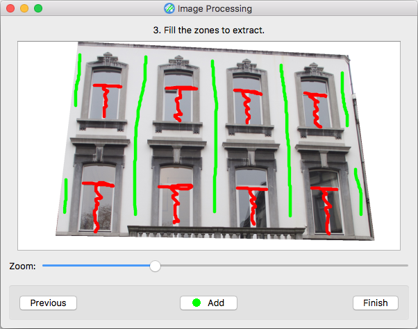
However, some material can interfer with the algorithm. To tell the algorithm to not take into account some material, use the red pencil to erased them.
If many photos were selected in order to be extracted, you will be invited to start again at step 1 with the next image, etc.
At the end of the processing, you will be redirected to the main window.
Manage masks
Masks can be a more precise way to select the facade surfaces of the buildings.
A masks is a image with black and white pixels. When we associate a mask to an original image, the mask will be placed at the top of the original image, and all the pixels of the original image below a black pixel of the masks will be erased. A mask can then be used to remove parts of an original image.
Export a mask.
To export the mask of an image, this image must have been processed beforehand (to process an image, please refer to the Extract colors section).
Once the image is processed, double-click on the image in the Imported Images window. A new window appears containing the original image and the mask resulting of the cutting process. If the image at the right is only white, that means the processing had not been done yet.
Click on the Export mask button to save the mask in your computer.
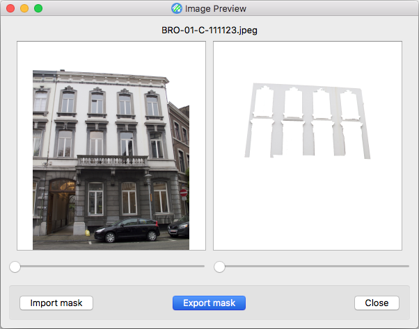
The two sliding bars allow you to zoom on the two pictures.
To close the image preview and go back to the main window, click on the Close button.
Export a mask.
To export a mask, double-click on an image on the Imported Images window. The Image Preview window appears. Click on the Export mask button to export a black and white mask to the computer.
You can also use the Export retoured image button to export the image filtered with the mask.
Import a mask.
To import a mask, double-click on an image on the Imported Images window. The Image Preview window appears. Click on the Import mask button to load a black and white mask from the computer.
Once the mask imported, the image at the right is the result of the mask on the original image (at the left).
Get statistics
Once all the wanted images have been processed, the main purpose of this application is to get statistical information about them.
To get these pieces of information, select the images you want to get statistics and click on the Get the graphs button in the main window.
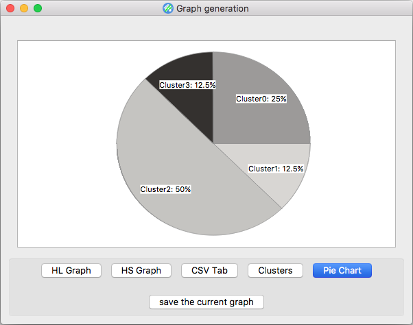
A new window will appear. This is the Graph generation window. This window is composed of an information area and 6 buttons.
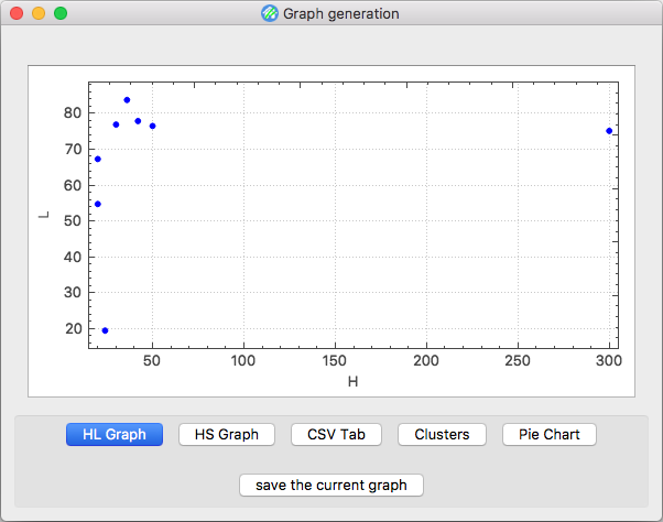
HL graph
HL graph, the first button, shows the colors coordinates of the processed images you selected in the HL space (from the HSL colorimetric space). You can explore the HL graph by maintaining left-click on the image and by scrolling the window in order to zoom.
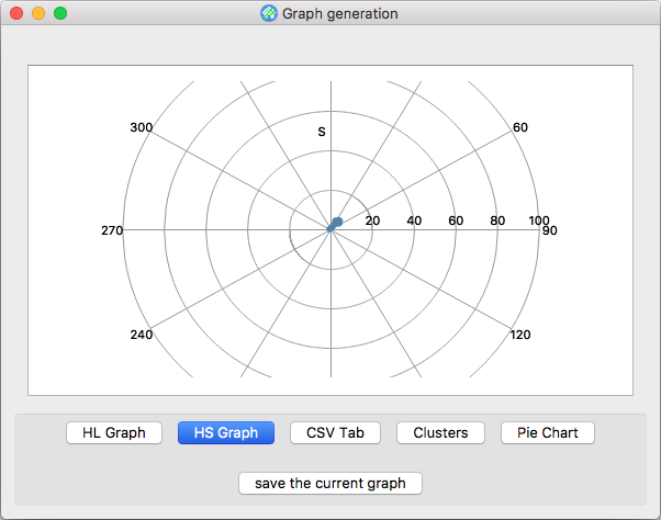
HS graph
Hs graph, the second button, shows the colors coordinates of the selected images in the HS space. You can explore the HS graph by maintaining left-click on the image and by scrolling the window in order to zoom.
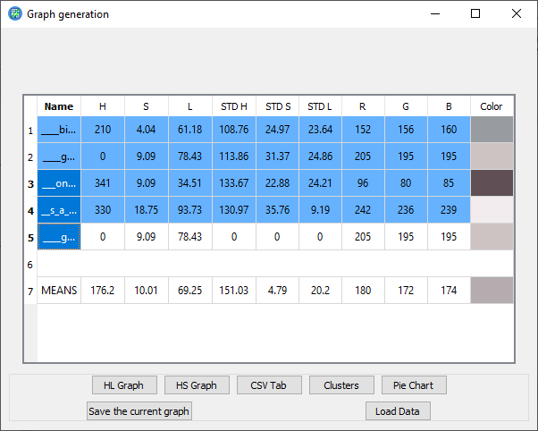
CSV Tab
The third button CSV Tab displays a table containing the summury of the colors coordinates of the seleted images. This table includes the names, the HSL values of the colors, the standard deviations amongst all the processed colors, the corresponding RGB value, and a color preview.
The last row of that table is the mean of all the processed colors.
The light blue lines are the images that are currently selected. You can select other images by clicking on the rows that you want to select. Use ctrl+click and shift+click to select multiples images. The rows highlighted in dark blue are the rows that you are selecting, and that will be use to draw the graphs when you change tab.
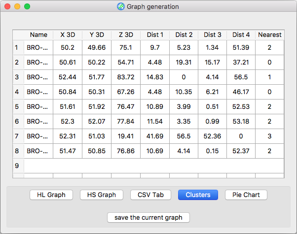
Clusters
The fourth button Clusters splits all the colors in four clusters due to a kmeans algorithm according to their 3D coordinates in the 3D space. There will be 4 centroids (from 1 to 4), one per cluster. A color is associated to a centroid if the distance between this color and this centroid is smaller than the distance from this color to the other centroids.
In this way, the program can gather all the colors into 4 sets and get the mean colors of the 4 clusters.
At the end of the table, the coordinates of the 4 centroids are represented in various colorimetric spaces: 3D, CIE L*a*b*, RGB, and HSL.
Pie Chart
Pie Charts, the fifth button, represents the data from the 4 centers using a Pie Chart. Each center is represented by its mean color and by the pourcentage of the number of colors it has inside its cluster. You can explore the Pie Chart by maintaining left-click on the image and by scrolling the window in order to zoom.
Save a graph
Save the current graph, the last button, allows you to save the current graph or table (displays on the screen) to the computer into a png image. In the CSV tab, it will save CSV file of the selected images that you can re-import later.
Change the language
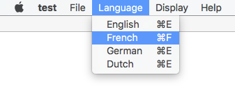
The application is translated into four different languages: english, french, german and dutch. To switch from one language to another, click on the Language tab and select the desire language.
Additional information
If a problem occurs during a step, or if you have any questions, please ask by mail through the Contact section.
Thank you.